HPC HW POWER MONITORING: POWER MONITORING SYSTEMS¶

HIGH DEFINITION ENERGY EFFICIENCY MONITORING (HDEEM)¶

Overview¶

HDEEM is an out-of-band power monitoring technology developed by Bull (now Atos) and integrated into their production HPC systems. It provides comprehensive, high-frequency power measurements across all major hardware components without imposing computational overhead on user applications.

Deployment Context¶

HDEEM is available on:

Bull Sequana - Atos’s modern HPC system family
Bullx B7xx series - Previous generation systems
Integrated directly into the motherboard firmware (BMC - Baseboard Management Controller)

Power Measurement Domains¶

HDEEM captures power at multiple granularity levels:

Blade-Level Measurement (1 kHz sampling):

Entire blade power consumption
Captures total power across all components
Suitable for system-level accounting and facility management

Voltage Regulator (VR) Monitoring (100 Hz sampling):

CPU - Processor power rails
DRAMs - Memory subsystem power
NIC* - Network interface power (where available)
VAUX* - Auxiliary power rails (where available)

The higher granularity at 100 Hz allows detailed component-level analysis while the 1 kHz blade measurement captures transient behavior.

Accuracy and Reliability¶

Measurement Uncertainty: ±2%

This is exceptional accuracy for production systems
Enables reliable energy accounting and charge-back models
Suitable for research requiring high-precision measurements

Software Interface¶

HDEEM provides both C library APIs and command-line utilities for data collection:

Command-line Tools:

startHdeem - Initiate power measurement collection
stopHdeem - End measurement and store data
checkHdeem - Verify measurement status
printHdeem - Export collected data in human-readable format
clearHdeem - Reset measurement buffers

Integration Model:

Out-of-band collection (no application overhead)
Post-execution data retrieval
Scriptable for automated monitoring workflows

INTEL RUNNING AVERAGE POWER LIMIT (RAPL)¶

Architecture Overview¶

RAPL is Intel’s in-band power monitoring and power capping mechanism built into modern x86 processors. It provides per-domain power measurement and enforcement capabilities at the hardware level, enabling both measurement and active power management.

Access Interface¶

Linux Interface:

/sys/devices/virtual/powercap/intel-rapl/intel-rapl:X/intel-rapl:0:Y

This sysfs interface allows user-space tools to:

Read energy consumption counters
Query power limits
Set new power caps (with appropriate privileges)
Monitor domain-specific measurements

Power Domains¶

RAPL defines multiple independent power control domains, each with distinct characteristics:

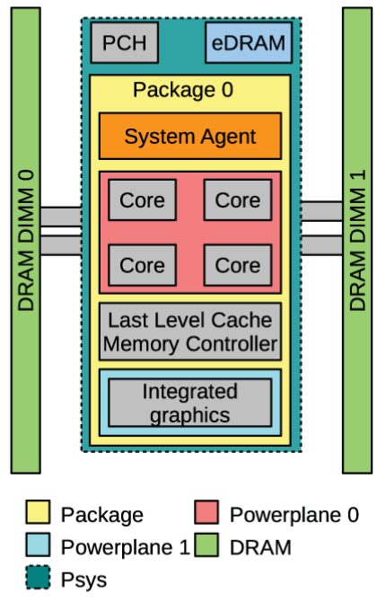
Package Domain

Encompasses entire CPU package: cores + uncore components (caches, memory controller, interconnects)
Dual Time Window Architecture:
- Short window: 1.2 × TDP, ~milliseconds resolution (captures transient peaks)
- Long window: 1 × TDP, ~second resolution (enforces sustainable power budget)
Use case: Preventing thermal runaway and managing peak power draw

DRAM Domain

Controls memory subsystem power consumption
Availability: Server architectures only (not available on client CPUs)
Single time window - Simpler control model than Package domain
Default State: Disabled by default; must be explicitly enabled
Use Cases:
- Memory-intensive workload characterization
- P-State scaling coordination
- Data center power budgeting

PP0 / Core Domain

Restricts power limits to CPU cores only (excluding uncore)
Single time window - Fixed control window
Modern Availability: Not available on newer server architectures (implementation dropped)
Use case: Disaggregating core vs. uncore power contributions

PP1 / Graphics Domain

Controls integrated GPU power (iGPU on client processors)
Server Availability: Not applicable - no integrated graphics on server CPUs
Single time window
Use case: Laptop/desktop power optimization

PSys / Platform Domain (Skylake and newer)

Controls entire System-on-Chip power
Dual time window (short + long, like Package domain)
Architecture Requirement: Skylake and newer Intel architectures
Vendor Support: Requires explicit firmware support; not universally available
Use case: System-wide power budgeting across all domains

Domain Relationships¶

These domains form a hierarchy: $$P_{\text{Package}} = P_{\text{PP0}} + P_{\text{PP1}} + P_{\text{Uncore}}$$

For older CPUs with distinct domains, the relationship enables component-level analysis.

INTEL RAPL: MSR REGISTERS AND ENERGY ACCOUNTING¶

Model-Specific Registers (MSRs)¶

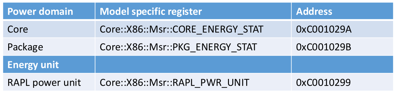
RAPL measurement and control are implemented through dedicated CPU model-specific registers (MSRs) that require privileged access. Applications access these registers through the msr kernel module on Linux or specialized libraries.

Power Limit Configuration¶

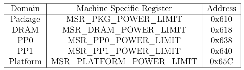
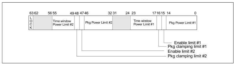
MSR_PKG_POWER_LIMIT (0x610) - Package Power Cap Settings

Defines both short-term and long-term power limits for the CPU package
Structure contains two independent limit windows
Controls hardware power throttling mechanisms
Enables dynamic power budget enforcement

Unit Conversion MSRs¶

Energy measurements from RAPL counters are stored in raw hardware units that must be converted to physical units using calibration factors:

MSR_RAPL_POWER_UNIT (0x606) - Unit Conversion Factors Contains conversion multipliers for:

Power units - Converts raw counts to Watts
Energy units - Converts raw counts to Joules
Time units - Converts time window encodings to seconds

These are system-specific constants determined at CPU design time and stored in read-only register fields.

Energy Status Registers¶

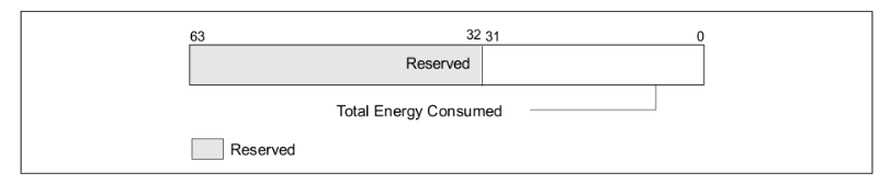
Each domain maintains an energy accumulator that wraps around periodically. Reading the register reports total energy consumed since last wrap-around or CPU reset.

Domain Energy Counters:

MSR_PKG_ENERGY_STATUS (0x611) - CPU Package energy (cores + uncore)
MSR_DRAM_ENERGY_STATUS (0x619) - Memory subsystem energy
MSR_PP0_ENERGY_STATUS (0x639) - Core-only energy (excludes uncore)
MSR_PP1_ENERGY_STATUS (0x641) - Graphics domain energy
MSR_PLATFORM_ENERGY_COUNTER (0x64D) - Entire SoC energy (Skylake+)

Energy Accounting Method¶

Energy consumption is computed by:

Baseline Reading: Read energy counter at time $t_0$ $$E_0 = \text{read}(\text{MSR_PKG_ENERGY_STATUS})$$
Post-Execution Reading: Read counter at time $t_1$ $$E_1 = \text{read}(\text{MSR_PKG_ENERGY_STATUS})$$
Raw Energy Difference: $$\Delta E_{\text{raw}} = E_1 - E_0 \text{ (with wraparound handling)}$$
Convert to Joules: $$E_{\text{Joules}} = \Delta E_{\text{raw}} \times \text{unit_factor}(\text{MSR_RAPL_POWER_UNIT})$$

Practical Considerations¶

Counter Wraparound:

Energy counters are typically 32-bit fields and wrap around
Wraparound interval typically 60-100 seconds depending on power draw
Monitoring software must poll frequently enough to detect wraparound

Accuracy Limitations:

RAPL estimates energy based on performance counters and power models
Typical accuracy: ±5-10% compared to external power meters
Estimates vary with workload characteristics and CPU frequency scaling

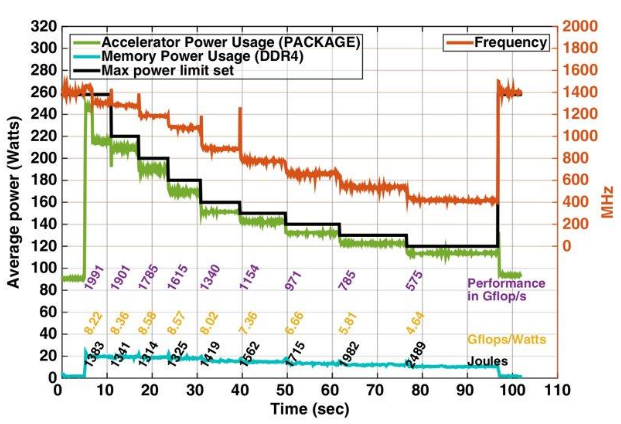
Reference: Haidar et al: “Investigating power capping toward energy-efficient scientific applications” - Foundational work on RAPL behavior and characterization

Haidar et al: Investigating power capping toward energy-efficient scientific applications

AMD RAPL¶

Compatibility and Design¶

AMD implements a compatible but simplified variant of Intel’s RAPL interface. The key differences reflect AMD’s architectural choices and market positioning:

Compatibility Layer:

Same sysfs interface as Intel RAPL for software compatibility
Allows existing monitoring tools to work across vendors with minimal modification
Reduces software development and testing burden for HPC centers

Operational Scope¶

Energy Reporting Only:

AMD RAPL is read-only for energy consumption measurement
Does NOT support power capping - no enforcement mechanism
Fundamental architectural difference from Intel’s dual measurement+control design

This reflects AMD’s philosophy of letting the operating system and BIOS handle power management rather than exposing hardware capping mechanisms.

Power Domains¶

Package Domain (PKG)

Encompasses all in-socket components:
- CPU cores (all cores combined)
- IO die containing I/O controllers and interconnects
- Other socket-level components
Monolithic measurement - no separation between core and uncore like older Intel systems
Reflects AMD Zen architecture with integrated IO die design

Core Domain

Per-core granularity - Each CPU core can be measured independently
Modern Zen architecture provides core-level power instrumentation
More detailed than Intel’s package-level approach for core analysis
Use case: Identifying power imbalance across cores, vectorization efficiency

Architectural Implications¶

AMD’s integrated IO die design eliminates the traditional core/uncore split:

Can’t separately measure memory controller power (integrated into IO die)
Can’t separately measure interconnect power
Simplifies hardware design but reduces measurement granularity

Software Support¶

Access through the same Linux sysfs interface as Intel, enabling:

Tool portability across AMD and Intel systems
Unified monitoring scripts
Vendor-neutral application code

Reference: [1]: https://github.com/amd/amd_energy/issues/1 - AMD Energy driver implementation details

FUJITSU A64FX¶

Architecture Context¶

The Fujitsu A64FX is a custom ARM-based processor designed specifically for HPC, featuring:

ARM SVE (Scalable Vector Extension) for floating-point performance
High memory bandwidth optimized for scientific computing
Purpose-built power monitoring infrastructure

This processor powers Fugaku, one of the world’s leading supercomputers.

Power Measurement Architecture¶

Unlike x86 systems dominated by Intel/AMD, the A64FX implements a highly granular, cycle-accurate power monitoring system tailored to scientific workload analysis.

Power Domains¶

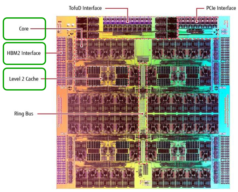
Core Domain

Individual processor core power consumption
Per-core instrumentation enables load balancing analysis
Identifies vectorization efficiency by core behavior

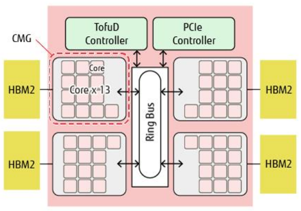
Memory Domain - Core Memory Group (CMG)

Local memory subsystem per core group
Captures memory hierarchy power (hierarchical memory design)
Reflects Fujitsu’s multi-level memory architecture
Important for data-intensive workload profiling

L2 Cache Domain (LLC)

Level 2 cache (Last-Level Cache in the core complex)
Separate power measurement for cache hierarchy
Enables cache-focused optimization studies
Critical for bandwidth-bound application analysis

Sampling Characteristics¶

Cycle-Accurate Measurement:

Sampling Frequency: Every cycle of the domain
Essentially continuous measurement with zero delay
Unprecedented temporal resolution compared to x86 systems
Enables detailed transient power behavior analysis

Implications for Research:

Can correlate power spikes with exact instruction sequences
Identify power efficiency at instruction level
Characterize vectorization overhead and efficiency
Fine-grained workload power signature analysis

Use Cases¶

Vectorization Analysis - Understand SVE instruction efficiency
Memory Hierarchy Optimization - Optimize access patterns for memory power
Power Model Development - Create detailed power models for HPC workloads
Dynamic Power Management - Real-time frequency/voltage scaling decisions

TBD	TBD

NVIDIA GPU POWER MONITORING¶

NVIDIA Management Library (NVML)¶

NVML is NVIDIA’s primary API for GPU monitoring and management, providing programmatic access to GPU power metrics. It works across all NVIDIA GPU architectures (consumer and data center).

Power Measurement Functions¶

Total Energy Consumption:

NvmlDeviceGetTotalEnergyConsumption(device)

Returns cumulative energy consumed by GPU since power-on or reset
Measured in millijoules (mJ)
32-bit counter that wraps around periodically
Use case: Post-execution energy accounting for batch jobs

Instantaneous Power Usage:

NvmlDeviceGetPowerUsage(device)

Current GPU power draw in milliwatts (mW)
Sampled at typical ~100ms intervals
Direct reading from GPU power management unit
Use case: Real-time power monitoring and dynamic adaptation

Multi-Field Power Query:

NvmlDeviceGetFieldValues(device, [GPU_POWER, MEMORY_POWER, ...])

Efficient bulk reading of multiple power domains simultaneously
Reduces API overhead compared to individual calls
Returns vector of power values in one operation

Power Domains¶

GPU_POWER

Compute unit power (shader cores, tensor cores)
Represents arithmetic compute resource power

MEMORY_POWER (sub-domain)

HBM (High Bandwidth Memory) or GDDR memory subsystem
Includes memory controllers and interconnects
Distinct measurement from compute power

MODULE_POWER (Grace Hopper, Grace Blackwell)

CPU+GPU co-processor module power
Captures heterogeneous compute power
New domain for Grace architecture

Command-Line Interface¶

Quick Power Check:

nvidia-smi --query-gpu=power.draw --format=csv

Outputs:

Current power consumption per GPU
Format: comma-separated values (one per GPU)
Useful for shell scripts and monitoring loops

Example Output:

power.draw
150.00 W
142.00 W

Architectural Notes¶

NVML works across all GPU types: discrete, data center, consumer
Power measurements are estimates based on hardware models
Typical accuracy: ±5-10% (similar to RAPL)
Sampling resolution: ~100ms typical interval
No energy counter wraparound with modern NVIDIA drivers

Limitations¶

Cannot access per-core or per-SM (Streaming Multiprocessor) power
Limited to GPU power; system interconnect power not measured
Requires NVIDIA driver with NVML support
GPU-only monitoring; does not include host CPU power
Command-line utility
- Instant power: nvidia-smi –query-gpu=power.draw –format=csv

AMD GPU POWER MONITORING¶

AMD System Management Interface (AMD SMI)¶

AMD provides AMD SMI (formerly AMD ROCm SMI) as their GPU monitoring and management API, mirroring NVIDIA’s NVML approach but with AMD-specific implementations.

API Functions¶

Total Energy Consumption:

amdsmi_get_energy_count(device)

Cumulative energy consumed by GPU
Energy value in joules (J)
Counter behavior similar to NVIDIA’s energy counter
Use case: Batch job energy accounting

Current Power Usage:

amdsmi_get_power_info(device)

Instantaneous power draw
Returns power value and timestamp
More detailed than simple instant power reading
Includes power limit information

Access Control¶

Group Membership Requirements: To access GPU power metrics, users must be members of:

video group - Access to GPU hardware
render group - Access to rendering/compute capabilities

This security model:

Prevents unprivileged users from querying GPU power (privacy)
Allows HPC centers to control who can monitor hardware
Differs from NVIDIA’s approach which may allow broader access

Command-Line Interface¶

Instant Power Query:

amd-smi metric --power

Outputs current power consumption across all AMD GPUs accessible to user.

Typical Output:

GPU[0]: 120 W
GPU[1]: 135 W

Comparison with NVIDIA¶

Aspect	AMD SMI	NVIDIA NVML
API	amdsmi_* functions	Nvml* functions
Energy	amdsmi_get_energy_count	NvmlDeviceGetTotalEnergyConsumption
Power	amdsmi_get_power_info	NvmlDeviceGetPowerUsage
Access Control	video, render groups	Depends on driver/OS
Multi-domain	Limited	Memory_power domain
Granularity	GPU-level	GPU + Memory domains

Implementation Notes¶

AMD SMI maintains API compatibility where possible with NVIDIA’s NVML
Power measurements use GPU firmware counters and power models
Sampling resolution: ~millisecond range (hardware-dependent)
Supports AMD RDNA and CDNA GPU architectures
Limited domain separation compared to NVIDIA’s multi-domain support
Command-line utility
- Instant power: amd-smi metric –power

NVIDIA GRACE CPU POWER MONITORING¶

Architecture Context¶

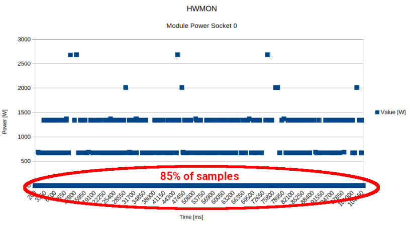
NVIDIA GRACE is a high-performance ARM-based CPU designed for HPC and data centers. Unlike NVIDIA’s GPU-focused NVML library, GRACE CPU power monitoring uses Linux’s standard HWMON (Hardware Monitoring) interface, reflecting its role as a CPU rather than a co-processor.

HWMON Interface¶

Linux HWMON provides standardized hardware monitoring through sysfs:

Power Measurement Files:

/sys/class/hwmon/hwmon*/device/power1_average
/sys/class/hwmon/hwmon*/device/power1_average_interval

Generic, vendor-agnostic interface
Works across different CPU types and manufacturers
Text-based file I/O for easy integration
Kernel-level access (typically requires root or special permissions)

Measurement Characteristics¶

Sampling Window:

Interval: 50-1000 milliseconds (configurable via power1_average_interval)
Longer than RAPL’s sub-millisecond resolution
Trade-off: Lower overhead but coarser temporal resolution

Reported Value:

Average power over the measurement window
NOT energy accumulation (no counter)
Each read gives mean power during interval: $P_{\text{avg}} = \frac{\text{Energy}}{\text{Interval}}$

Calculation for Energy: To compute energy from average power readings: $$E = P_{\text{avg}} \times \Delta t$$

Where $\Delta t$ is the measurement window duration.

Power Domains¶

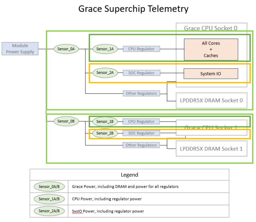
GRACE partitions CPU power into distinct measurement domains:

Grace Domain (Total)

Entire CPU package power
Encompasses all sub-domains
Reference point for other measurements

CPU Domain

Compute cores and core-local resources
Represents active computation power

SysIO Domain

System IO controllers and interconnects
Memory controllers
Off-CPU infrastructure power

DRAM Domain

Memory subsystem power
Main memory and cache hierarchy

Domain Relationships¶

The domains maintain a hierarchical accounting relationship: $$P_{\text{Grace}} = P_{\text{CPU}} + P_{\text{SysIO}} + P_{\text{DRAM}}$$

This decomposition enables:

Identifying whether power consumption is compute-bound or memory-bound
Understanding infrastructure overhead
Optimizing specific subsystems

Practical Implications¶

Measurement Overhead:

HWMON is lower overhead than RAPL on some systems
50-1000ms window trades temporal resolution for simplicity
Suitable for longer-running jobs where millisecond precision unnecessary

Integration:

No special library required (plain sysfs reading)
Shell scripts can directly monitor: cat /sys/class/hwmon/.../power1_average
Enables easy integration into existing monitoring infrastructure

NVIDIA GRACE HOPPER / GRACE BLACKWELL¶

Heterogeneous Architecture¶

NVIDIA’s Grace Hopper (and upcoming Grace Blackwell) represent a paradigm shift: CPU+GPU co-processors integrated on a single module. This creates unprecedented challenges and opportunities for power monitoring.

Unified Module Architecture¶

Module-Level Design:

Single coherent computing system combining CPU and GPU
Shared memory hierarchy and fast interconnects
Requires unified power monitoring across heterogeneous domains
Enables genuine heterogeneous computing (not discrete GPU+CPU)

Power Domains¶

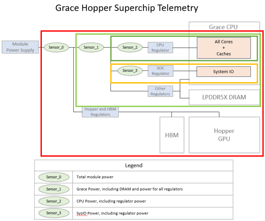
Grace Hopper power monitoring exposes multiple layers of domain decomposition:

Module Domain (Top-level)

Total power consumption of entire Grace Hopper co-processor
Includes all CPU, GPU, and interconnect power
Reference point for system-level accounting

Grace CPU Domain

CPU cores + SysIO + DRAM combined
Represents CPU-side power consumption
Derived from Grace CPU’s three-component model

CPU Domain

CPU compute cores only (cores themselves)
Excludes system infrastructure
Fine-grained CPU analysis

SysIO Domain

CPU-side system controllers and interconnects
Includes chipset and interconnect logic

GPU Domain

Hopper GPU accelerator power (Module - Grace)
Derived by subtraction from total module power
Represents heterogeneous accelerator consumption

Domain Hierarchy and Accounting¶

$$P_{\text{Module}} = P_{\text{Grace}} + P_{\text{GPU}}$$

$$P_{\text{Grace}} = P_{\text{CPU}} + P_{\text{SysIO}} + P_{\text{DRAM}}$$

Measurement Access¶

Dual Interface Support:

HWMON (Hardware Monitoring)
- Linux standard interface via sysfs
- Available for all domains
- Lower-level, kernel-integrated access
NVML (NVIDIA Management Library)
- NVIDIA’s high-level API
- More refined data structures
- Better integration with NVIDIA ecosystem tools
- Same functions as discrete GPUs but with CPU awareness

Use Cases¶

Workload Characterization:

Identify if bottleneck is CPU or GPU: compare $P_{\text{CPU}}$ vs $P_{\text{GPU}}$
Understand heterogeneous load balance
Optimize task distribution across CPU and GPU

Power Budgeting:

Allocate power budgets to CPU and GPU independently
Prevent one component from monopolizing power budget
Enable dynamic load balancing under power constraints

System Efficiency Analysis:

Identify infrastructure overhead (SysIO power)
Optimize interconnect usage
Understand memory subsystem power contribution

Challenges¶

Attribution Complexity:

GPU domain often derived (subtraction) rather than directly measured
Potential accumulation of measurement error
More difficult to achieve high accuracy in heterogeneous systems

Interface Consistency:

HWMON and NVML may report slightly different values
Need careful validation and understanding of differences
Important for reproducible research

POWER MONITORING IN PRACTICE: LUMI SUPERCOMPUTER¶

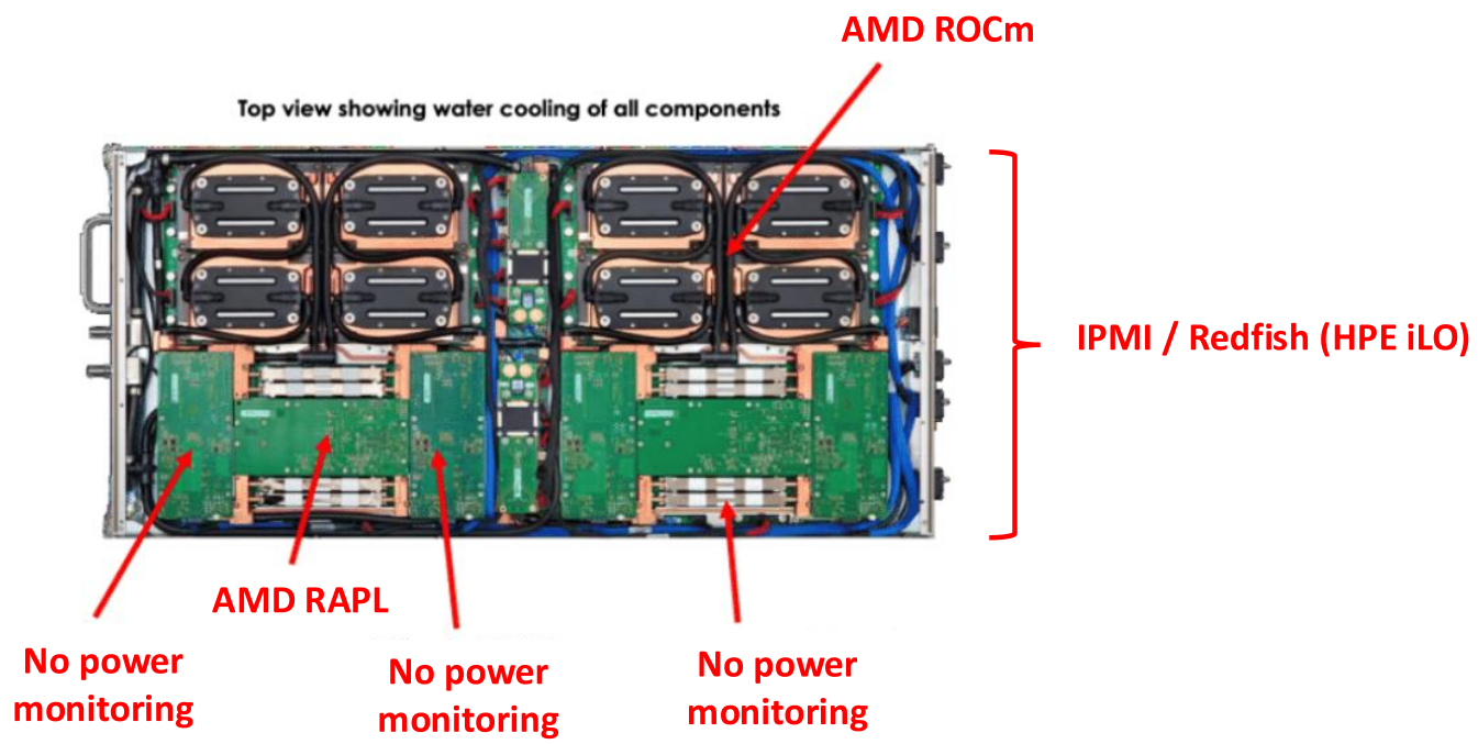
Real-world power monitoring implementation requires balancing theoretical capabilities with practical constraints. The LUMI supercomputer (hosted in Finland) provides an instructive case study of how these monitoring systems are deployed in production HPC environments.

Integrated Monitoring Stack¶

LUMI combines multiple power monitoring technologies:

RAPL - CPU-side power measurement
NVIDIA NVML - GPU/accelerator power (where applicable)
HDEEM or vendor systems - Node-level baseline
PDU monitoring - Facility-level accounting

Real System Challenges¶

The following visualization shows actual power baseline data from LUMI:

Key observations from production data:

Variability in idle power baseline
Complex relationship between components
Need for system-specific calibration

POWER BASELINE¶

The Measurement Challenge¶

As discussed in detail in the introduction, power monitoring systems have inherent measurement gaps:

High Frequency Energy Measurement of Some Components (e.g., RAPL, NVML)

Provides detailed measurements of CPU and GPU power
Missing energy consumption of the remaining parts (memory controllers, interconnects, infrastructure)

Low Frequency Power Monitoring of the Whole Node (e.g., HDEEM, PDU)

Captures total node power
Unreliable energy measurement for short and medium length regions (high relative error)

Node Power Baseline Estimation¶

To estimate power consumption of non-monitored on-node components, researchers use empirical calibration:

Load the node with a uniform, reproducible workload (e.g., synthetic benchmark like LINPACK or STREAM), then develop an energy model that accounts for unmeasured components:

Model Development Equation: $$P_{\text{node}} = P_{\text{measured}} + P_{\text{baseline}} + P_{\text{overhead}}$$

Where:

$P_{\text{measured}}$ = Component power from RAPL/NVML
$P_{\text{baseline}}$ = Idle system overhead
$P_{\text{overhead}}$ = Unmeasured component contribution

System-Specific Calibration¶

Critical Principle: Power baseline is system-specific and must be evaluated for each system individually because:

Hardware Variation - Different processors, memory types, interconnects
Firmware Differences - BIOS settings, power management policies
Environmental Factors - Cooling efficiency, ambient temperature
Workload Sensitivity - Unmonitored components respond differently to different workloads

Practical Implementation¶

Once baseline is established:

Use it consistently across all experiments on that system
Document baseline methodology for reproducibility
Re-evaluate if hardware changes are made
Account for seasonal variations in data center conditions

KAROLINA SUPERCOMPUTER: POWER BASELINE CASE STUDY¶

Real systems demonstrate the complexity and system-specificity of baseline determination. The Czech supercomputer Karolina provides a detailed real-world example with distinct node types requiring separate baseline analysis:

Node Types and Power Profiles¶

Karolina’s heterogeneous architecture includes different node configurations:

ACN - Accelerated Compute Nodes

Include GPU accelerators (typically NVIDIA)
Higher peak power consumption
Complex power relationships between CPU and GPU

CN - Compute Nodes

CPU-only nodes
Simpler power behavior
Different baseline characteristics

Baseline Determination Visualization¶

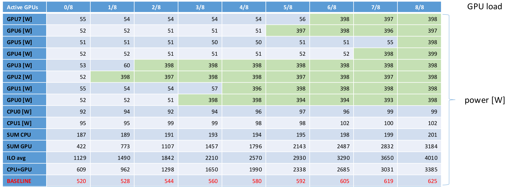
../../_images/26-baseline-Karolina-ACN.png

../../_images/26-baseline-Karolina-CN.png

Key Insights from Real Data¶

These visualizations demonstrate:

Different Baselines per Node Type
- ACN and CN nodes show distinctly different baseline power profiles
- Cannot use single system-wide baseline
- Requires node-type-aware monitoring
Non-Linear Power Relationships
- Power doesn’t scale linearly with load
- Overhead varies with workload type
- Multiple calibration points needed
Infrastructure Overhead
- Significant portion of idle power is infrastructure (cooling, power delivery)
- Changes with system age and environmental conditions
- Must be factored into charge-back models

Practical Implications for Karolina Users¶

Use ACN baseline for accelerated jobs
Use CN baseline for CPU-only jobs
Monitor outliers (jobs with unusually high power)
Re-calibrate seasonally or after hardware changes
Understand baseline uncertainty when reporting energy metrics

This real-world example illustrates why power monitoring in production HPC systems requires careful, ongoing calibration and validation beyond theoretical models.