HPC HW POWER MONITORING: ITRODUCTION
ENERGY
Understanding Power vs Energy
Energy consumption is one of the most critical metrics in HPC systems, but it’s important to distinguish between power and energy:
Power (measured in Watts [W]) is the instantaneous rate at which energy is being consumed at a specific moment in time
Energy (measured in Joules [J] or Watt-hours [Wh]) is the total amount of work performed over a period of time
The relationship between them is captured by this fundamental formula:
$$Energy = Power \times Time$$
$$E [J] = P [W] \times \Delta t [s]$$
Practical Examples
To make this concrete, consider these conversions:
$$1 \text{ Watt} \times 1 \text{ second} = 1 \text{ Joule}$$ $$1 \text{ Watt} \times 1 \text{ hour} = 1 \text{ Watt-hour (Wh)} = 3,600 \text{ Joules}$$
Why does this matter for HPC? A system drawing 100 kW for just 10 minutes consumes significantly less energy than one drawing 50 kW continuously for 1 hour, even though the latter has lower peak power. In HPC centers and data halls, understanding this relationship is essential for:
Estimating cooling requirements
Budgeting operational costs
Optimizing job scheduling and workload distribution
Reducing carbon footprint
Measurement Approaches
Energy can be measured through different sampling methods, each with trade-offs:
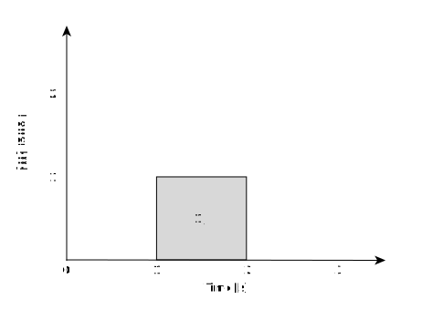
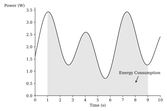
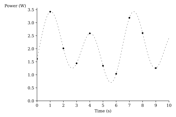
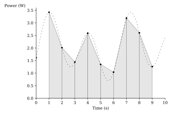
The visualization below illustrates three common approaches to estimate total energy from power samples:
TBD |
TBD |
Blade (HDEEM) samples [W] |
|---|---|---|
|
|
|

POWER MONITORING
Power monitoring in HPC systems occurs at multiple hierarchical levels, each serving different purposes in understanding where energy is consumed and how to optimize it.
Monitoring Hierarchy
The monitoring stack extends from individual hardware components up to entire data centers:
On-Node Component Level (most granular):
CPU - Processor cores and their power states
ACC - Accelerators (GPUs, specialized processors)
Memory - DRAM and cache subsystems
NIC - Network interface cards
This level provides the highest granularity but requires access to hardware performance counters or specialized monitoring interfaces.
System-Level Monitoring (broader scope):
Node - Entire compute node aggregated power
Chassis - Multiple nodes in an enclosure (e.g., blade servers)
PDU - Power Distribution Unit monitoring at infrastructure level
Data Center and Infrastructure (facility perspective):
Rack - Power consumption of an entire rack
System - The complete HPC system
Data Hall - Entire data center
Building - Facility-wide energy accounting
HPC System Examples
Different HPC centers implement power monitoring across their infrastructure to meet various needs:
HPE Cray |
OLCF Frontier |
OLCF Frontier |
|---|---|---|
|
|
|
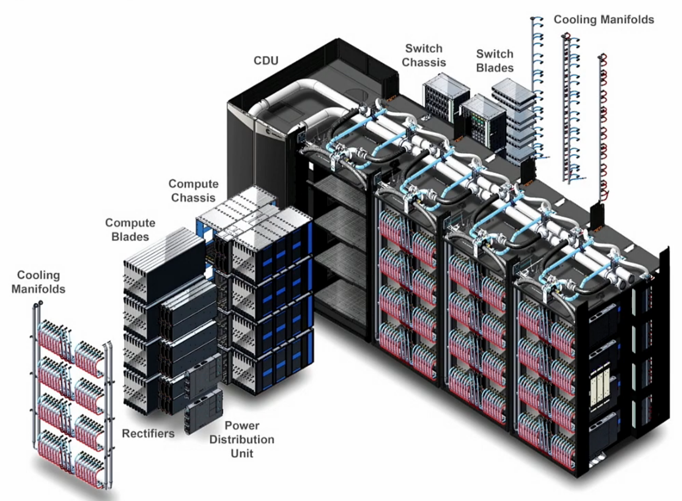
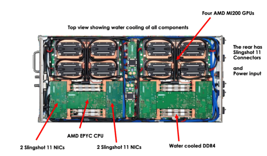
Design Considerations
Why monitor at multiple levels?
Accountability - Charge-back models and resource allocation require node-level or job-level energy metrics
Optimization - Component-level data reveals which parts consume most power (e.g., memory vs. compute)
Reliability - Infrastructure monitoring helps detect cooling problems and power delivery issues
Predictive Maintenance - Facility-level trends can indicate aging equipment or degradation
Workload Characterization - Understanding which jobs/users consume most energy enables scheduling optimization
Each monitoring level introduces different trade-offs between precision, overhead, cost, and actionability.
POWER MONITORING SYSTEMS FOR HPC
Modern HPC power monitoring systems vary widely in their implementation approach, each with distinct advantages and limitations suited to different deployment scenarios and requirements.
Key Dimensions of Variation
Power monitoring systems differ across several critical dimensions:
Data Source - Whether measurements come from hardware sensors, performance counters, PDU devices, or infrastructure meters
Accessibility - Whether data is accessible directly to users (in-band) or only to system administrators (out-of-band)
Temporal Resolution - Sampling frequency from milliseconds to seconds to minutes
Spatial Granularity - Component-level vs. node-level vs. system-level aggregation
Computational Overhead - The cost of monitoring itself and impact on application performance
Accuracy - Measurement precision and reliability across different workloads
Integration Complexity - Whether the system requires custom hardware modifications or uses existing infrastructure
Cost - Capital investment and operational expenses
Comparative Analysis
The following visualization compares leading power monitoring systems used in HPC centers:

System Selection Criteria
When choosing a power monitoring system for an HPC facility, consider:
Use Case - Are you tracking individual jobs, optimizing node efficiency, or managing facility-wide power budgets?
Scale - Does your system need to monitor 10 nodes or 10,000?
Accessibility Requirements - Do users need real-time access, or is post-execution reporting sufficient?
Integration with Existing Infrastructure - Can you leverage vendor-provided monitoring, or do you need custom solutions?
Accuracy Tolerance - Is ±5% accuracy acceptable, or do you need ±1%?
Time-to-Deployment - Can you wait for development, or do you need immediate deployment?
Different HPC centers make different choices based on their specific operational constraints and research goals.
IN-BAND AND OUT-OF-BAND POWER MONITORING
One of the most fundamental architectural decisions in power monitoring systems is whether measurements should be accessible to end users (in-band) or restricted to system administrators (out-of-band). This choice has profound implications for system design, overhead, and usability.
In-Band Monitoring
Definition: Power data is accessible directly to users and applications during execution, typically through programming APIs or command-line interfaces.
Characteristics:
Vendor Specific - Usually implemented by hardware manufacturers (Intel, AMD, NVIDIA) and tightly integrated with their architectures
HW Performance Counters - Leverages built-in CPU/GPU counters and registers designed for performance analysis
Read from User-Space - Applications can query power metrics directly without privileged kernel access in many cases
Real-time Access - Users can monitor their jobs while they run and make adaptive decisions
Advantages:
Enables adaptive power management - applications can adjust behavior based on power consumption
Low overhead - measurements are typically fast register reads
Easy integration - can be embedded directly in application code
Immediate feedback - researchers can experiment with optimization strategies in real-time
Disadvantages:
Limited to vendor implementations - not all architectures are equally well-supported
May not capture complete system power (e.g., memory subsystem, interconnects)
Potential security concerns - users can observe power consumption patterns of other applications
Accuracy varies - estimates based on models rather than direct hardware measurements
Out-of-Band Monitoring
Definition: Power measurements are collected independently of application execution and accessible only to system administrators or through post-execution reporting.
Characteristics:
No Overhead to Applications - Monitoring infrastructure operates independently, adding zero computational overhead
High Overhead of Exposing to User-Space - Significant effort required to collect, store, and expose data to users
Custom Sensors - Often uses specialized hardware devices (power meters, PDU monitoring, thermal sensors)
Post-Execution Reporting - Users typically receive energy metrics after jobs complete
Advantages:
Zero application impact - no interference with computational work
Complete observability - can measure entire node/chassis power including all components
Security isolation - power data doesn’t leak between users or applications
Highly accurate - direct hardware measurements rather than estimates
Infrastructure-centric - enables facility-level power budgeting and management
Disadvantages:
No real-time feedback - users cannot adapt during execution
Higher capital cost - requires specialized hardware infrastructure
Deployment complexity - integration challenges with existing systems
Limited granularity - typically node-level rather than component-level insights
Comparative Analysis: RAPL vs DiG
Two contrasting approaches in modern HPC are illustrated below:
RAPL |
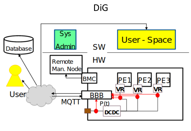
DiG |
|---|---|
|
|
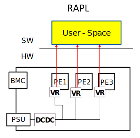
RAPL (Running Average Power Limit) - Intel’s in-band solution providing user-accessible power measurements through performance counters on modern processors. Applications can query energy consumption in real-time with minimal overhead.
DiG (Distributed iDirect Gauge) - An out-of-band approach using dedicated monitoring hardware to capture complete system power without impacting application execution.
Design Trade-Off Matrix
Dimension |
In-Band |
Out-of-Band |
|---|---|---|
User Access |
Direct |
Post-execution reporting |
Application Overhead |
Low |
Zero |
Measurement Completeness |
Partial |
Complete |
Real-time Adaptation |
Yes |
No |
Deployment Complexity |
Low |
High |
Cost |
Low |
High |
Accuracy |
Moderate |
High |
Practical Guidance
Choose In-Band monitoring when:
Your research focuses on power-aware algorithms and adaptive optimization
You need real-time feedback for interactive exploration
Hardware budget is limited
Application performance impact must be minimized
Choose Out-of-Band monitoring when:
You need accurate facility-wide power accounting
Component-level energy breakdown is critical
Security and isolation are primary concerns
You’re building infrastructure for long-term operational management
NODE POWER BASELINE
The Energy Attribution Challenge
A fundamental problem in HPC power monitoring is the measurement gap: hardware components have heterogeneous instrumentation coverage. While some parts (like CPU cores) provide high-frequency power measurements through performance counters, many critical components lack direct monitoring.
The Measurement Hierarchy Problem
Consider a typical compute node:
High Frequency Energy Measurement of Some Components (millisecond resolution)
CPU cores (via RAPL, MSR counters, or similar)
Some GPU memory (via nvidia-smi on some hardware)
Individual accelerators (where vendor support exists)
Missing Energy Consumption of the Remaining Parts (no direct measurement)
Memory controllers and their power management logic
System interconnects (PCIe, InfiniBand, Ethernet)
Power conversion and delivery circuitry
Cooling and thermal management subsystems
Motherboard chipset and I/O controllers
Low Frequency Power Monitoring of the Whole Node (second to minute resolution)
PDU-level measurements
Baseboard Management Controller (BMC) readings
Out-of-band monitoring systems
The Estimation Gap
This creates a critical measurement problem:
$$\text{Unmeasured Components} = \text{Total Node Power} - \sum \text{Measured Components}$$
For short to medium-length jobs (seconds to minutes):
Component-level measurements show what the CPU/GPU consumed
Whole-node measurements show total consumption
The difference can be highly variable and unreliable to estimate
This makes short- and medium-length energy measurements unreliable without additional calibration.
Node Power Baseline Estimation Method
To estimate power consumption of non-monitored on-node components, researchers use an empirical calibration approach:
Procedure:
Idle Node Measurement - Measure total node power when fully idle (all cores parked, no computation)
Controlled Load Experiments - Load the node with a uniform, reproducible workload
Run synthetic benchmarks that stress all components uniformly
Common choices: LINPACK (HPL), STREAM, or specialized benchmarks
Measure at multiple power levels to create a calibration curve
Model Development - Construct a simple energy model: $$P_{\text{node}} = P_{\text{baseline}} + P_{\text{cpu}} + P_{\text{unmonitored}}$$
Where $P_{\text{unmonitored}}$ can be estimated from the difference between measured and actual consumption.
Validation - Test the model against diverse real workloads to verify accuracy
System-Specific Nature
Critical insight: Power baseline is system-specific and must be evaluated for each system individually because:
Hardware variation - Different manufacturers, component vendors, and firmware versions have different overhead profiles
BIOS/firmware settings - Power management policies, thermal thresholds, and voltage regulators vary significantly
Environmental factors - Temperature, voltage supply variations, and cooling efficiency affect measurements
Workload interaction effects - Unmonitored components consume power based on unmeasured metrics (memory bandwidth, I/O traffic, thermal management activity)
Measurement Instruments and Examples
The following visualizations show real-world power baseline measurement data and instrumentation:
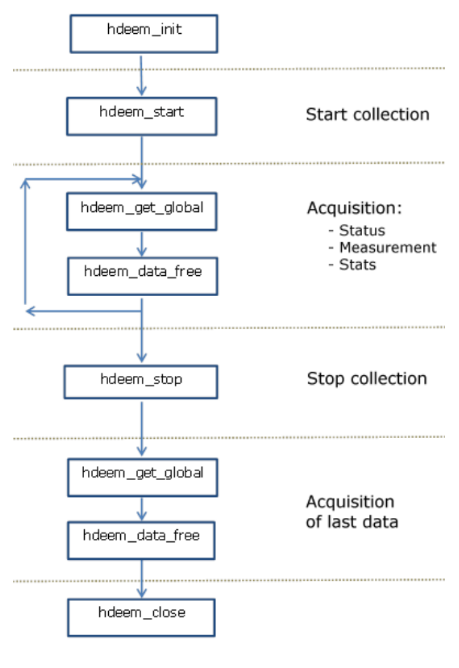
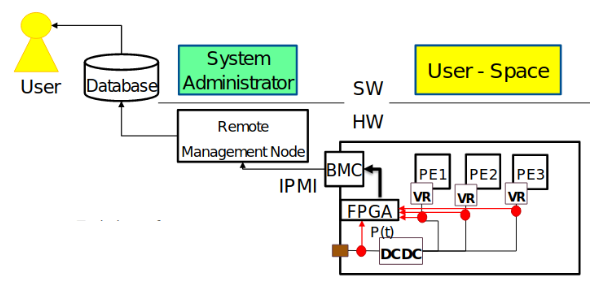
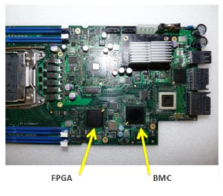
HDEEM (High Definition Energy Efficiency Monitoring) - A specialized out-of-band monitoring system that captures detailed power metrics at high frequency and enables accurate baseline determination through controlled experiments.
Practical Implications
When using energy measurements in your research:
Understand the coverage - Know what percentage of your node’s power is directly measured vs. estimated
Design for accuracy - Run long-enough jobs that baseline variations become negligible relative to computation time
Validate your assumptions - Compare model predictions against actual measurements for your workloads
Document your methodology - Report which components are measured, which are estimated, and how the baseline was determined
Use baselines consistently - Once established for a system, reuse the same baseline across experiments for reproducibility